Inside the Infinity Engine

A fractal renderer can fail long before it runs out of iterations. It can fail at the addition that constructs a pixel coordinate.

let center = -0.743643887037151
let pixelOffset = 1.0e-25
let moved = center + pixelOffset
// In ordinary Double arithmetic, moved == center.

The offset is representable. The sum is not distinguishable from the original center. Asking the GPU to calculate that same rounded coordinate several million times will produce an image quickly, but it will not recover the missing geometry.

Mandelbrot Metal 3’s Infinity Engine addresses this problem by dividing the numerical work. The CPU constructs a shared reference orbit in double-double arithmetic. Metal evaluates nearby pixels as small deviations from that orbit, using a fast Float tier and restarting difficult pixels in quad-single arithmetic. A bounded scheduler delivers the resulting image progressively while preserving the user’s current navigation state.

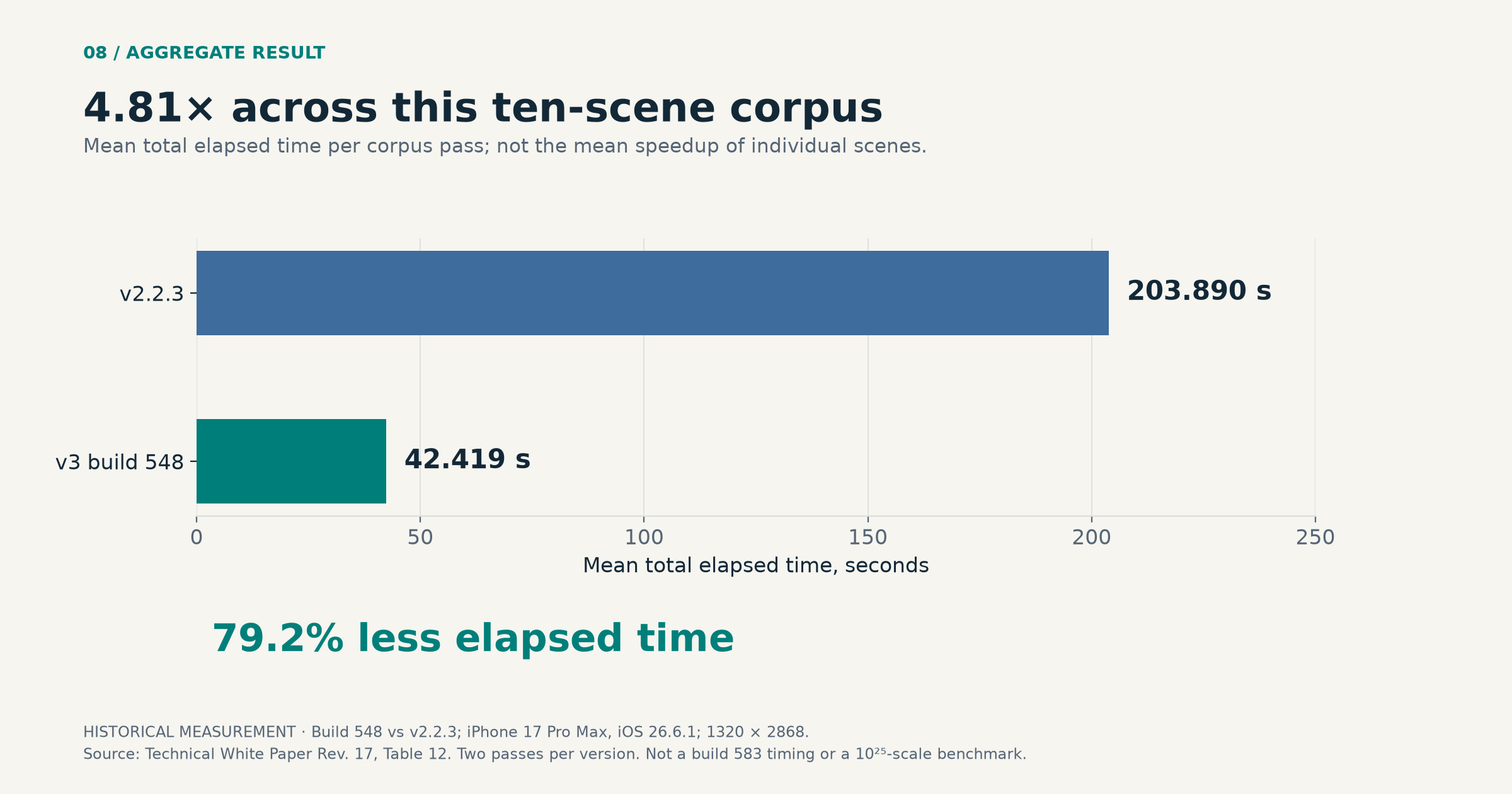
The published ten-scene physical-device benchmark reduced the mean total corpus time from 203.890 seconds to 42.419 seconds: a 4.81× aggregate speedup. That result belongs to Version 3 build 548 on one iPhone 17 Pro Max. The implementation examined here is build 583, reviewed on September 17, 2026. The older timings reflect the architecture, not fresh measurements of this newer build.

Version 3 is in preview as this article is prepared. Its public Mandelbrot scale ceiling is 10²⁵; useful detail remains dependent on the scene, iterations, arithmetic, and device. This article concerns that public rendering path. Experimental code beyond the ceiling does not claim support for a deeper range.

1. Precision is a pipeline property

For Mandelbrot rendering, each pixel selects a complex parameter c and evaluates

z₀ = 0
zₙ₊₁ = zₙ² + c

For this map, exceeding radius 2 establishes escape. Failing to escape within a finite iteration budget does not, in general, prove membership in the set. A black boundary pixel may simply require more iterations.

The coordinate problem precedes the recurrence. Let Sₚ be the viewport scale in UIKit points per complex-plane unit, and q the drawable’s pixels-per-point multiplier. Then

Sₓ = q · Sₚ             drawable pixels per complex-plane unit
h  = 1 / Sₓ            complex-plane distance between adjacent pixels

The distinction matters. The product’s navigation ceiling and a benchmark’s effective drawable scale use different units. At Sₚ = 10²⁵ and q = 3, adjacent pixels are approximately 3.33 × 10⁻²⁶ units apart.

Near a center of magnitude one, a rough absolute-coordinate significand requirement is

p ≈ log₂(Sₓ)

That is about 84.6 bits in the example above, before guard bits, orbit sensitivity, or a rounding-error margin. Binary64 has 53 significand bits. Its large exponent range does not solve the loss of a tiny increment when you add it to an order-one number.

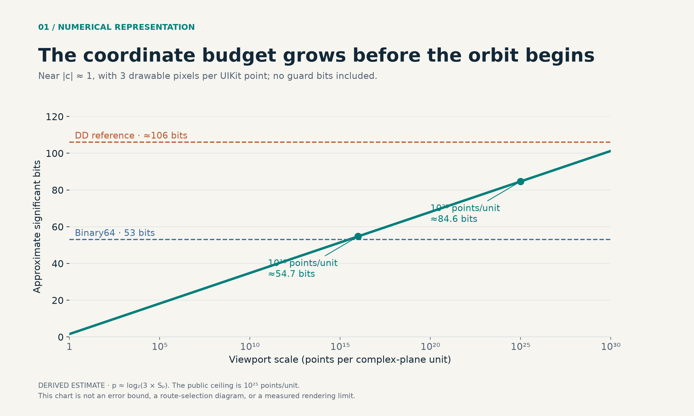
This is why precision cannot be repaired only inside a shader. Pan and pinch calculations, viewport commits, reference anchors, pixel mapping, bookmarks, and restoration must preserve the same small offsets. The current source keeps a compensated center and forms reference-relative offsets before reducing them to the GPU’s transport representation. A more accurate recurrence cannot recover coordinate bits discarded by an earlier state transition.

The public scale policy enforces one 10²⁵ ceiling across the application. A value stored in a wider internal representation is not, by itself, permission to render beyond that boundary.

2. Change the coordinate system of the computation

Choose a nearby reference parameter c₀. Compute its orbit once:

Z₀ = 0
Zₙ₊₁ = Zₙ² + c₀

For a pixel at c = c₀ + Δc, write zₙ = Zₙ + δₙ. Substitution gives

Zₙ₊₁ + δₙ₊₁ = (Zₙ + δₙ)² + c₀ + Δc
δₙ₊₁ = 2Zₙδₙ + δₙ² + Δc

The last line is an exact algebraic identity. Infinity retains δₙ². It does not replace the quadratic map with a first-order Taylor approximation.

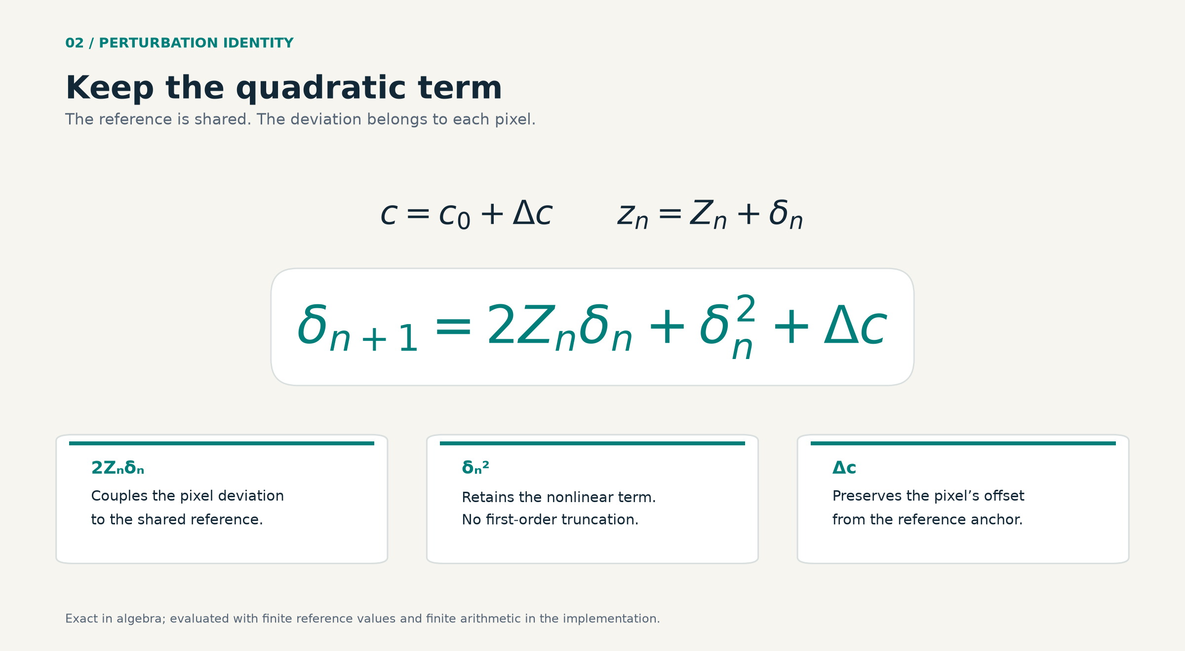
That distinction answers a common objection: how can Float calculations help at scales far beyond ordinary Float coordinate resolution? They operate on a small relative quantity. Representing a small Δc is a different problem from adding Δc to a large absolute c₀. The shared reference carries the large-scale orbit structure; each pixel tracks its departure from that structure.

The advantage is reuse. A direct deep renderer pays for extended-precision orbit arithmetic per pixel. Perturbation pays for a reference orbit and then executes many cheaper delta orbits in parallel. It does not magically eliminate the iteration loop. A difficult pixel can still require tens of thousands of updates.

A useful cost model is

Tframe ≈ Treference + Tfast pixels + TQS restarts
       + Trecovery + Tcolor/relief + Tscheduling/presentation

This is a decomposition, not a measured profile. Its purpose is to expose the costs a “GPU kernel time” alone would omit. Reference preparation, precision promotion, and presentation are part of the user’s wait.

3. Preserve the reference across the CPU/GPU boundary

On the CPU, double-double represents a value as an unevaluated sum of two binary64 components:

x = xhi + xlo

Normalized double-double arithmetic provides approximately 106 significant bits under its operating assumptions. It is finite precision. It is not IEEE binary128, and it is not an arbitrary-precision backend.

The reference builder receives a compensated complex anchor, starts from zero, and stores successive iterates. It stops if the anchor escapes; the renderer must then handle pixels whose useful orbit extends beyond that reference buffer.

Uploading one Float per component would discard most of the reference’s precision. Instead, the current Swift helper emits four Float limbs by repeatedly subtracting the component already emitted:

// Production helper, with its surrounding declarations omitted.
func ddFloatExpansion(_ value: DD) -> SIMD4<Float> {
    var residual = value
    var limbs = SIMD4<Float>(repeating: 0)
    for index in 0..<4 {
        let limb = Float(residual.hi)
        limbs[index] = limb
        residual = ddSub(residual, DD(Double(limb)))
    }
    return limbs
}

The important operation is the subtraction in DD arithmetic. Collapsing hi + lo to one Double first would already throw away information before the Float conversion.

Each complex reference point contains two aligned float4 values: four real limbs and four imaginary limbs. The payload is 32 bytes per stored iterate. A 50,000-point orbit therefore occupies 1,600,000 bytes, about 1.53 MiB, before other buffers and resources. This is a storage calculation, not a measured memory peak.

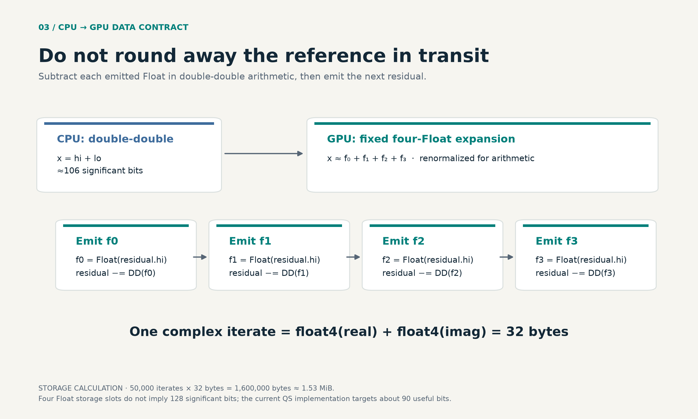
Metal reconstructs quad-single expansions from these limbs. The implementation describes approximately 90 useful significand bits for its QS operations. That is an implementation target, not a universal theorem about four Floats. Limb normalization, cancellation, range limits, and the exact sequence of operations all matter.

One multiplication primitive uses a rounded product and an FMA residual:

const float product = a * b;
const float residual = fma(a, b, -product);

Under the appropriate rounding and range assumptions, this is the basis of an error-free product transform. Expansion addition and multiplication combine residuals and renormalize them into a fixed number of limbs. The QD literature explains this family of multiple-component arithmetic; Infinity adapts the approach to Float/FMA operations in Metal.

The assumptions deserve attention. Algebraic identities alone do not establish the behavior of compiled floating-point code. Reassociation, contraction, underflow, and fast-math options can change numerical properties. The reviewed Xcode project enables Metal fast math; the source-level residual formula should therefore not be read as a blanket proof of strict IEEE behavior for the compiled kernel. Compiled arithmetic needs its own validation against higher-precision references and difficult inputs.

4. Adapt precision per pixel—and restart when necessary

Always using QS would be straightforward, but it would make every pixel pay the expensive path’s cost. Infinity first attempts Float perturbation while keeping the pixel parameter relative to the reference anchor.

For a non-escaped fast-path iterate, the current kernel checks two conditioning indicators:

large delta:
|δ|² > max(10⁻³⁰, 0.0625 · |Z|²)

cancellation:
|Z|² > 10⁻²⁰  and  |Z + δ|² < 10⁻⁶ · |Z|²

It also rejects non-finite states. These are numerical heuristics; they are not a certified forward-error bound. A large relative deviation weakens the local representation, while a reconstructed orbit much smaller than its reference signals cancellation.

If the fast attempt returns a miss, the QS routine starts again from iteration zero. It does not simply convert the current Float state into four limbs and continue. Widening an already rounded trajectory would preserve its accumulated error more accurately; it would not undo it.

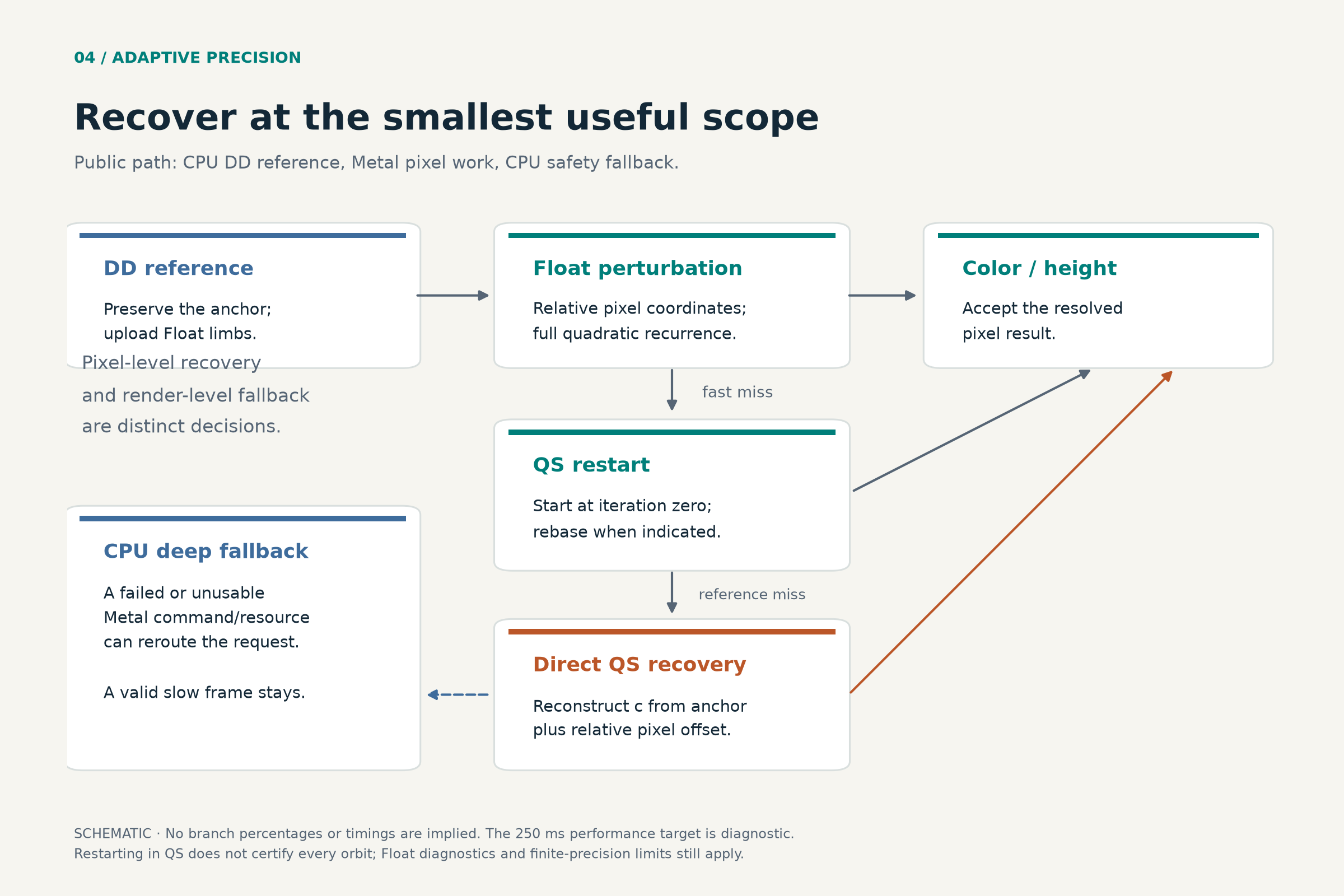
QS perturbation can rebase its current state. In the implementation, rebasing assigns the reconstructed orbit to the deviation and resets the reference index to zero. Because Z₀ = 0, the deviation can represent the entire current orbit. The next quadratic update then advances it using the same parameter offset.

This rebase changes the representation a pixel uses. It does not ask the CPU to build a new reference halfway through that pixel. Constructing a new reference for a committed viewport is a separate operation.

The QS path uses different growth and cancellation thresholds: a relative squared-delta factor of 0.25 and a reconstructed/reference squared-magnitude ratio of 10⁻⁷. Its diagnostics and escape/color values are reduced to Float even though the recurrence uses expansions. A more accurate recurrence state does not make every decision in the pipeline a QS decision.

If the reference becomes exhausted or unusable, the public path can restart as a direct QS Mandelbrot calculation. It reconstructs c from the uploaded anchor plus the relative pixel offset, avoiding a return to the less precise absolute coordinate mapping. A failed or unusable Metal command can instead route the request to the established CPU deep renderer.

This is an adaptive architecture with recovery paths, not a guarantee that every boundary sample is correctly classified. That stronger claim would require an error analysis and validation regime beyond the presence of heuristics.

5. Schedule for a usable application, not just a fast dispatch

The benchmark drawable contains 1320 × 2868 = 3,785,760 pixels. At a 47,550-iteration maximum, a hypothetical full-budget pass would attempt roughly 180 billion pixel-iterations. Actual work depends on escape, restarts, and recovery. The multiplication nevertheless explains why one monolithic command can be a poor unit of interactive work.

The current live scheduler partitions the public Infinity frame into 128-row regions with up to three columns. The column count is

columns = max(1, min(3, floor(width / 256)))

It sorts tiles by distance from the image center, then submits bounded batches. At the benchmark dimensions, this produces 3 columns × 23 rows = 69 tiles, with the final row shortened to 52 pixels. Three tiles per batch gives 23 batches. These counts describe the current scheduler at those dimensions; they are not a claim that the historical build used this identical layout.

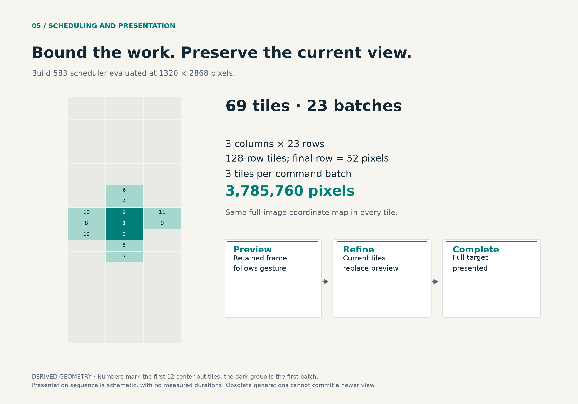
During a gesture, the last completed image follows the interaction transform. That gives immediate visual feedback, but it is a preview—not a newly evaluated deep frame. On commit, completed tiles progressively replace an initialized preview.

Every render request also carries a generation identity. If a new viewport supersedes a request, successful old work must not overwrite the new view. Numerical correctness and state correctness meet here: a beautifully computed tile from the wrong viewport is still the wrong output.

This produces three distinct latency questions: how quickly input affects the preview, how soon the first refined region appears, and how long the full requested frame takes to complete. A benchmark should say which one it measures.

The 250 ms performance target is another important distinction. The current policy records a missed target separately from runtime fallback. A valid slow frame is retained. Failure, invalid timing, or another unusable result can open the fallback circuit. Discarding a correct, completed GPU frame just to start a slower CPU calculation would add work without fixing its latency.

6. Coloring, relief, and capture remain part of the workload

Escape iteration alone is not the final image. The renderer reconstructs the orbit, computes a smooth escape coordinate, applies contrast and palette lookup, and writes color. The primary pass combines orbit evaluation with this color work; the app does not retain a general escape buffer for instant palette-only recoloring.

With 3D Look enabled, the current renderer also writes an R32Float height field. A second pass reads neighboring heights and estimates surface normals through central differences. A one-pixel halo around a tile supplies the neighboring samples needed at its edges. This lets relief shading read a completed field instead of recalculating four complete neighboring orbits for each shaded pixel.

The distinction between main-orbit cost and post-processing cost matters when comparing versions. Several benchmark scenes use 3D Look, and the current implementation has changed since that benchmark. The historical totals do not isolate the cost or benefit of today’s relief pipeline.

Capture is a separate complete render, including Canvas Size. It snapshots the composition and recomputes mapping and precision eligibility for the output dimensions. A larger output has a smaller complex-plane pixel step, so qualifying the live canvas does not automatically qualify a high-resolution export. Tiles use full-image coordinates to preserve continuity.

The public Infinity path requests one sample per pixel. Ordinary rendering paths can use larger sampling grids. Matching dimensions without matching sampling, iterations, palette, contrast, and lighting is not a controlled comparison.

7. The benchmark: what improved, and by how much

The following measurements come from Table 12 and Section 15.4 of the Mandelbrot Metal 3 Technical White Paper, Revision 17. These are published physical-device results, reproduced here; this article did not include a new device timing run.

The test used Release builds with separate bundle identifiers for v2.2.3 and v3.0 build 548, on an iPhone 17 Pro Max running iOS 26.6.1. The foreground, window-attached Metal surface was 440 × 956 points at 3× scale, producing a 1320 × 2868 drawable. High Quality Idle was off; Infinity used one sample per pixel. Bookmark-specific iterations, appearance, fractal family, and Julia parameter were retained.

Timing began immediately before applying each bookmark state and ended after the complete command path, including reference preparation, recurrence, color/lighting, final blit, and presentation submission. Launch and drawable-readiness waiting were excluded. This is an application-to-presentation-submission interval, not a measurement of display scanout or touch-to-photon latency.

Each version ran the corpus once forward and once in reverse. The table shows the published means and speedups; the companion CSV preserves both passes, effective scales, iteration limits, appearance, and routes.

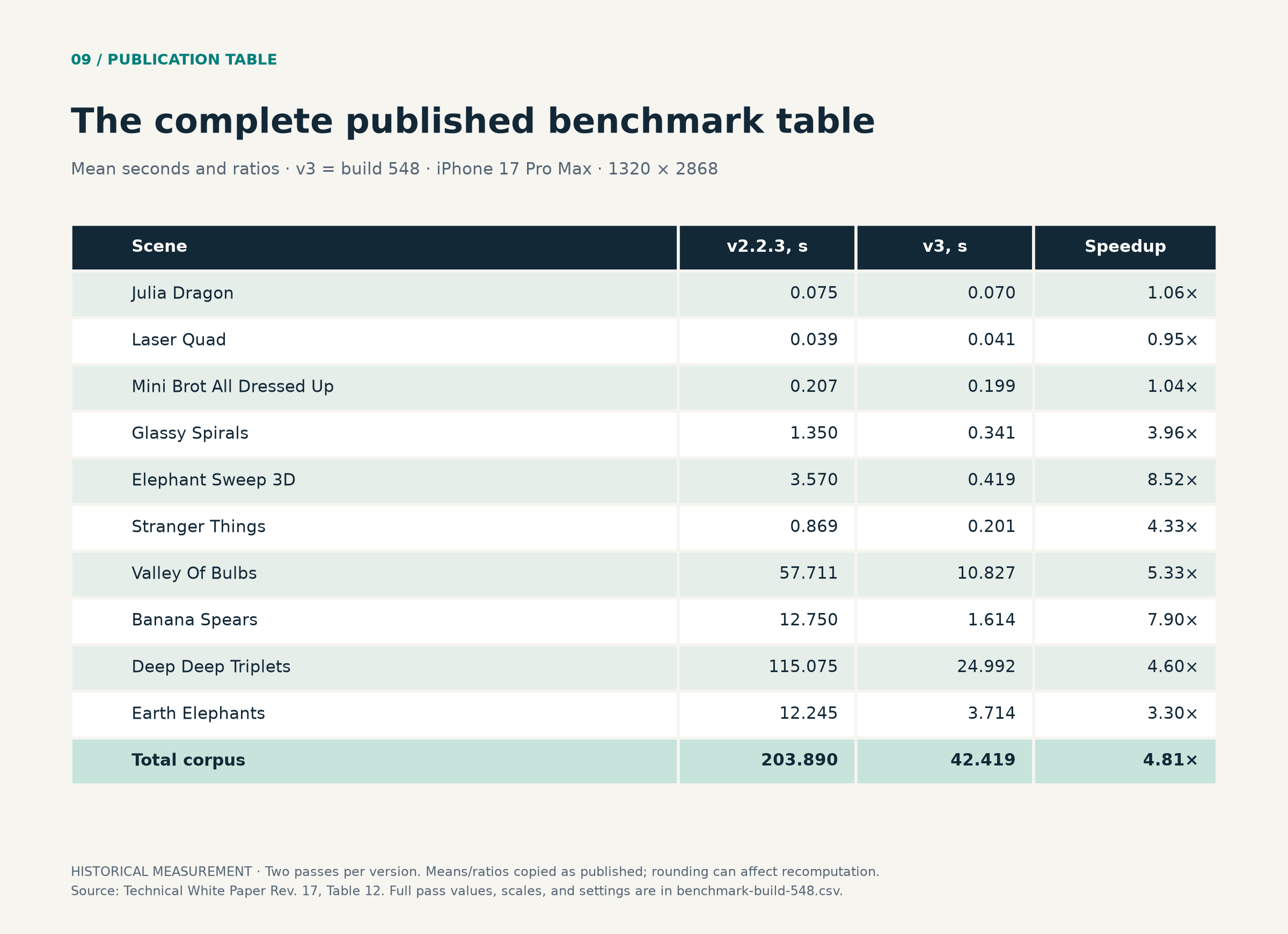
The paper calculated means and ratios from unrounded measurements. Its displayed values are rounded independently; recalculating from three-decimal values can produce small differences. The total is the mean total time of a ten-scene pass—not the average latency of one scene.

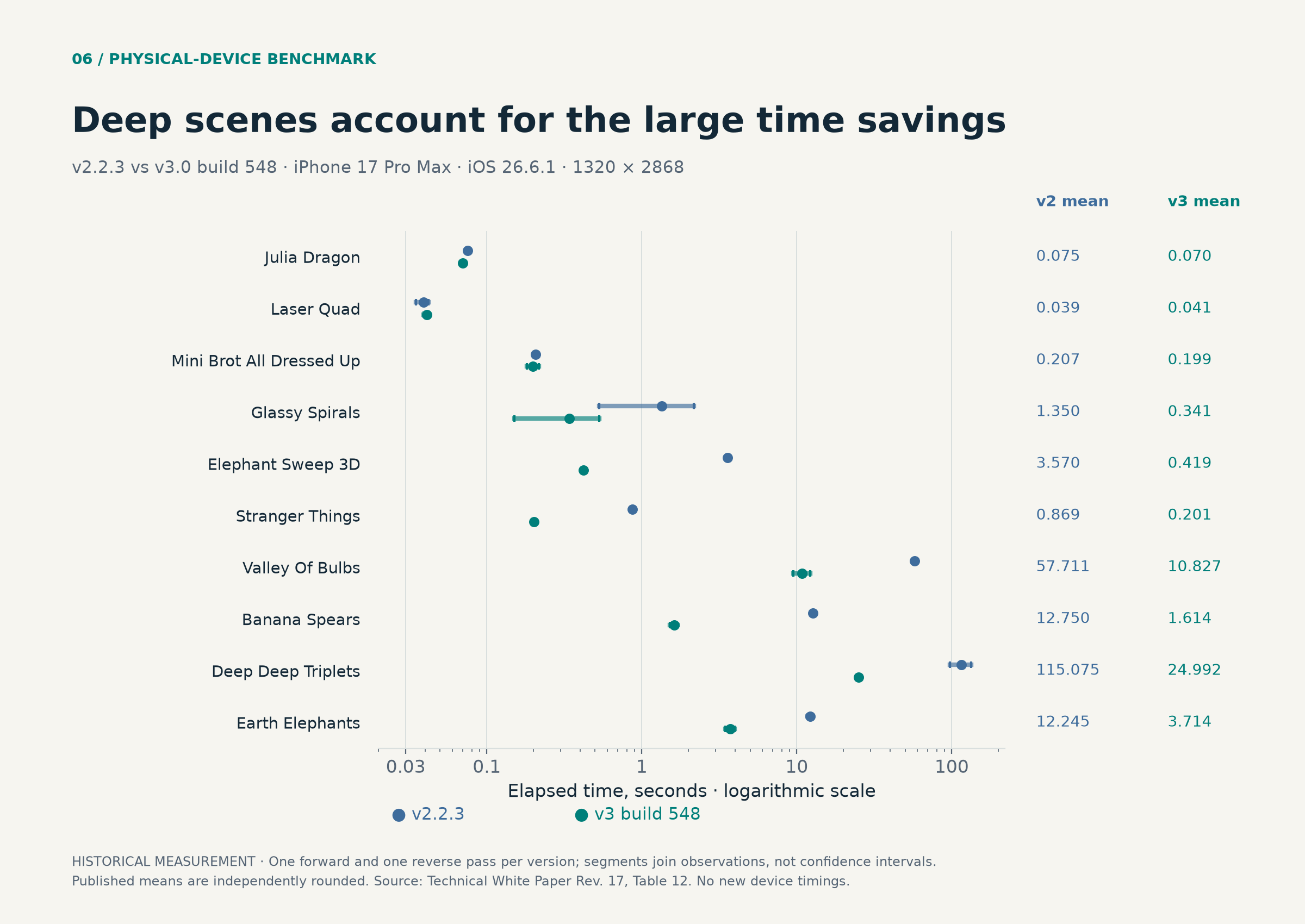
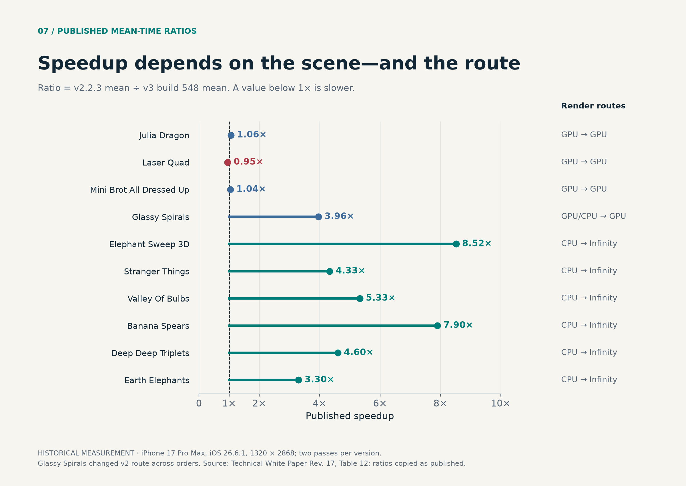
Six scenes changed from CPU to Infinity. Their published speedups range from 3.30× for Earth Elephants to 8.52× for Elephant Sweep 3D. Deep Deep Triplets contributes much more to elapsed-time savings than its ratio alone suggests: its reported mean fell by about 90.1 seconds.

The shallow GPU controls tell a different story. Julia Dragon and Mini Brot are close to parity. Laser Quad’s published ratio is 0.95×—about two milliseconds slower in v3. Glassy Spirals needs its own qualification: the v2 route changed between GPU and CPU across the two orders, while v3 stayed on GPU. Its 3.96× ratio is not an isolated measurement of the Infinity kernel.

The corpus ratio is

aggregate speedup = Σ mean(v2 scene time) / Σ mean(v3 scene time)
                  ≈ 203.890 / 42.419
                  ≈ 4.81×

elapsed-time reduction ≈ 1 − 42.419 / 203.890 ≈ 79.2%

It is not the arithmetic mean of ten speedup ratios. It weights expensive scenes more because they consume more of the total wait. Changing the corpus changes the aggregate.

Two observations per scene support a descriptive comparison, not a latency distribution. No defensible p95 or p99 estimate is possible here. Deep Deep Triplets ranged from 96.987 to 133.163 seconds on v2 and from 24.919 to 25.066 seconds on v3. Valley of Bulbs ranged from 9.491 to 12.164 seconds on v3. Order, thermal state, and scene-specific factors may contribute; these passes do not isolate causality.

The benchmark’s largest effective scale is 1.25 × 10¹⁵ pixels per unit. Consequently, the timing corpus does not measure performance at the 10²⁵ navigation ceiling. Depth qualification and performance qualification are related, but they are different evidence.

8. An image comparison is useful—and narrower than a proof

The published correctness comparison rendered Earth Elephants at 440 × 956, once with adaptive Float/QS routing and once with QS forced for every pixel. It found zero differing pixels and zero channel errors across 420,640 pixels.

That is valuable evidence that adaptive routing agreed with its control for this case. It does not establish independent mathematical correctness: the implementations share arithmetic and logic, and eight-bit output can hide differences that quantize to the same color. It also uses a smaller image than the physical-device timing corpus.

A stronger qualification program combines independent high-precision orbit references with cancellation-heavy scenes, early reference escape, long iteration counts, and coordinates near the public ceiling. Compare escape decisions and smooth values before quantization, then compare final images with matched sampling and appearance.

Application regressions deserve equal attention: tiny pan increments must survive state commits; old tiles must not replace newer generations; a tile’s relief halo must match the full-image coordinate map; capture must finish independently of a changing live viewport. These are observable correctness properties, not merely interface polish.

9. The next bottleneck is shared work

The architecture creates several opportunities for further improvement: better reference reuse, stronger diagnostics, more effective reference selection, and safe iteration skipping. None should be credited to the current benchmark without its own measurement.

Block-linear approximation is one possible acceleration. A locally valid block can be represented schematically as

δout = A · δin + B · Δc

For two consecutive blocks, composition yields

Acombined = A₂ · A₁
Bcombined = A₂ · B₁ + B₂

The difficult part is deciding when a block is valid, bounding the omitted nonlinear behavior, and recovering when the bound fails. BLA is a future acceleration direction here, not the recurrence used to generate the published measurements.

Extending depth also requires more than raising a scale constant. Coordinate storage, reference precision, GPU dynamic range, delta transport, navigation, serialization, and validation must advance together. Arbitrary precision in the reference service can be useful, but a more precise reference cannot compensate for a lossy downstream interface. The public path described in this article remains adaptive finite precision through its enforced ceiling.

The Infinity Engine’s central design decision is to spend precision where it preserves information and parallelism where work repeats. A shared accurate orbit makes the pixels cheaper. Adaptive restarts protect difficult trajectories. Bounded scheduling and generation checks make that computation usable in an interactive application.

The reported benchmark shows a substantial improvement for the measured deep scenes. The next engineering step is to keep expanding that evidence: newer builds, more devices, harder coordinates, and complete output workflows—with numerical accuracy and time to a finished image measured together.

---

Sources and companion material

• Technical White Paper, Revision 17, especially Sections 15.3–15.4 and Table 12, for the historical benchmark and image comparison.
• Perturbation Rendering and GPU Pipeline for the application’s published engineering explanations.
• Hida, Li, and Bailey, Library for Double-Double and Quad-Double Arithmetic, for multiple-component arithmetic.
• Apple, Metal resources, including the Metal Shading Language specification, for language and floating-point behavior.
• Engineering roadmap for future work; roadmap items are not measured capabilities.

Implementation review: local Mandelbrot Metal 3.0 build 583 source, September 17, 2026. I checked named functions, policy values, and current scheduler details against that source. Benchmark figures reproduce the separate build 548 dataset; derived diagrams and storage/precision calculations are labeled as such.